Flow Matching (FM) and Rectified Flow models—powering visual backbones such as Stable Diffusion 3.5 and FLUX—owe their remarkable sampling speed and generation quality to a simple geometric choice: transporting Gaussian noise along straight, deterministic ordinary differential equation (ODE) paths. Yet the very determinism that makes Flow Matching fast at inference creates an immediate friction when we try to post-train these models with online Reinforcement Learning (RL). Policy gradient methods require two ingredients that a deterministic ODE lacks: stochastic exploration to discover higher-reward samples from the same prompt, and tractable transition probabilities $\log \pi_\theta(a_t \mid s_t)$ to compute importance ratios and KL regularization.
Over the past year and a half, research at the intersection of RL and Flow Matching has moved rapidly across four stages:
- importing LLM-style Group Relative Policy Optimization (GRPO) into continuous flow models via ODE-to-SDE conversion;
- cutting rollout overhead and localizing temporal credit assignment with sliding windows and trajectory branching;
- bypassing reverse-time SDE likelihoods altogether via forward-process optimization (DiffusionNFT) and stochastic optimal control (Adjoint Matching / RAM);
- wrapping continuous flow generators inside multi-turn Agentic RL loops capable of planning, visual inspection, and iterative self-correction.
These notes connect the full arc—starting from MDP and policy-optimization foundations, walking through the exact SDE derivation and PyTorch step implementation, mapping every major branch of Flow-GRPO and forward-process / SOC RL, and synthesizing how reasoning and agentic RL extend continuous flow models.
Notation Convention (Lipman FM vs. SD3.5 / Flow-GRPO): In the foundational Flow Matching literature, $t=0$ typically denotes noise and $t=1$ denotes clean data ($X_t = t X_1 + (1-t) X_0$). In contrast, Rectified Flow diffusion backbones (Stable Diffusion 3.5, FLUX) and RL papers such as Flow-GRPO adopt the diffusion-aligned convention where $t=1$ is pure Gaussian noise $x_1 \sim \mathcal{N}(0, I)$ and $t=0$ is clean data $x_0 \sim q$: $$x_t = (1-t)x_0 + t x_1, \qquad v_t = \frac{dx_t}{dt} = x_1 - x_0.$$ Reverse-time generation therefore integrates from $t=1$ down to $t=0$ with negative step sizes $\Delta t = t_{\text{prev}} - t \lt 0$. Throughout Sections 2–4 below, we stick consistently to this SD3.5 / Flow-GRPO convention so every drift sign, score relation, and PyTorch line matches without ambiguity.
RL Foundations: From MDP to GRPO
Before converting continuous ODEs into RL policies, it helps to trace why modern post-training converged on critic-free group-relative objectives—and where continuous visual generation inherits or breaks LLM assumptions.
Framing Iterative Generation as an MDP
As formalized by DDPO[1], an iterative generative process over discrete reverse steps $t \in \{T, T-1, \dots, 1\}$ forms a finite-horizon Markov Decision Process $(\mathcal{S}, \mathcal{A}, \rho_0, P, R)$:
- State $s_t \triangleq (c, t, x_t)$: the conditioning prompt $c$, current timestep $t$, and intermediate noisy latent $x_t$.
- Action $a_t \triangleq x_{t-1}$ (or $x_{t+\Delta t}$ in continuous time): the next denoised latent produced by the sampler.
- Policy $\pi_\theta(a_t \mid s_t) \triangleq p_\theta(x_{t-1} \mid x_t, c)$: the conditional transition distribution induced by the neural network at step $t$.
- Transition kernel $P(s_{t+1} \mid s_t, a_t) \triangleq (\delta_c, \delta_{t-1}, \delta_{x_{t-1}})$: completely deterministic once action $a_t$ is sampled.
- Initial distribution $\rho_0(s_0) \triangleq (p(c), \delta_T, \mathcal{N}(0, I))$: prompt sampled from dataset distribution and latent initialized from isotropic Gaussian noise.
- Sparse terminal reward $R(s_t, a_t)$: equal to $r(x_0, c)$ only at the final clean image $x_0$, and $0$ at every intermediate step.
Notice the core tension embedded in this MDP: every intermediate action $x_{t-1}$ receives zero immediate feedback, while the terminal reward $r(x_0, c)$ (from human preference models, OCR detectors, or VLM judges) only becomes observable once the entire trajectory finishes.
Policy Gradient and Importance Sampling
To maximize expected trajectory return $J(\pi_\theta) = \mathbb{E}_{\tau \sim \pi_\theta}[R(\tau)]$, the REINFORCE policy gradient uses the log-derivative identity $\nabla_\theta P(\tau \mid \pi_\theta) = P(\tau \mid \pi_\theta)\nabla_\theta \log P(\tau \mid \pi_\theta)$. Expanding $P(\tau \mid \pi_\theta) = \rho_0(s_0)\prod_{t} P(s_{t+1}\mid s_t, a_t)\pi_\theta(a_t \mid s_t)$ causes the policy-independent initial distribution and transition kernels to vanish under the gradient, yielding:
$$\nabla_\theta J(\pi_\theta) = \mathbb{E}_{\tau \sim \pi_\theta}\!\left[\sum_{t} \big(R(\tau) - b(s_t)\big)\,\nabla_\theta \log \pi_\theta(a_t \mid s_t)\right]$$where subtracting an action-independent baseline $b(s_t)$ preserves unbiasedness ($\mathbb{E}_{a_t \sim \pi_\theta}[b(s_t)\nabla_\theta \log \pi_\theta(a_t \mid s_t)] = 0$) while reducing gradient variance.
In visual generation, however, generating a batch of trajectories $\tau$ requires tens of forward passes through a multi-billion-parameter DiT plus expensive VLM or detector reward evaluations. Performing only a single gradient update per rollout batch wastes almost all compute. Importance Sampling resolves this via the measure-change identity:
$$\mathbb{E}_{x \sim p}[f(x)] = \int f(x)\,\frac{p(x)}{q(x)}\,q(x)\,dx = \mathbb{E}_{x \sim q}\!\left[\frac{p(x)}{q(x)}\,f(x)\right]$$Applying this to trajectories sampled from a cached behavior policy $\pi_{\theta_{\text{old}}}$ yields the off-policy surrogate gradient weighted by the per-step probability ratio $\rho_t(\theta) = \frac{\pi_\theta(a_t \mid s_t)}{\pi_{\text{old}}(a_t \mid s_t)}$. Because $\pi_\theta$ can perform multiple mini-batch epochs on the same rollout buffer, sample efficiency rises sharply—until $\pi_\theta$ drifts too far from $\pi_{\text{old}}$, causing $\rho_t(\theta)$ to explode in variance and destabilize updates. Bounding that step size is precisely what separates vanilla policy gradients from PPO and GRPO.
PPO, GAE, and Direct Preference Optimization
PPO[2] addresses both high variance and uncontrolled step sizes. First, it introduces a learned value critic $V_\psi(s_t)$ estimating expected future return and computes Generalized Advantage Estimation (GAE) from single-step TD residuals $\delta_t = r_t + \gamma V_\psi(s_{t+1}) - V_\psi(s_t)$:
$$\widehat A_t^{\text{GAE}(\gamma, \lambda)} = \sum_{k=0}^{T-1-t} (\gamma\lambda)^k \delta_{t+k}, \qquad \widehat A_t = \delta_t + \gamma\lambda\,\widehat A_{t+1}$$Tuning $\lambda \in [0, 1]$ smoothly interpolates between low-variance/high-bias TD(0) ($\lambda=0$) and unbiased/high-variance Monte Carlo returns ($\lambda=1$). In PyTorch (e.g., verl-style implementations), GAE is computed in a single reverse pass over the trajectory:
with torch.no_grad():
    nextvalues = 0.0
    lastgaelam = 0.0
    advantages_reversed = []
    gen_len = token_level_rewards.shape[-1]

    for t in reversed(range(gen_len)):
        delta = token_level_rewards[:, t] + gamma * nextvalues - values[:, t]
        lastgaelam = delta + gamma * lam * lastgaelam
        # Apply step/token mask if episodes have variable length
        nextvalues = values[:, t]
        advantages_reversed.append(lastgaelam)

    advantages = torch.stack(advantages_reversed[::-1], dim=1)
    returns = advantages + values
Second, PPO constrains the policy shift by clipping $\rho_t(\theta)$ to $[1-\epsilon, 1+\epsilon]$, combining clipped actor loss, clipped value loss, entropy bonus, and KL penalty against a reference policy $\pi_{\text{ref}}$:
$$\mathcal{L}_{\text{PPO}}(\theta,\psi) = \mathbb{E}_{\tau \sim \pi_{\text{old}}}\!\left[\frac{1}{T}\sum_{t=0}^{T-1}\Big(-\min\big(\rho_t(\theta)\widehat A_t,\, \operatorname{clip}(\rho_t(\theta),1-\epsilon,1+\epsilon)\widehat A_t\big) + c_V \ell_t^{\text{value}}(\psi) - c_H \mathcal{H}(\pi_\theta) + \beta\,D_{\text{KL}}(\pi_\theta \,\|\, \pi_{\text{ref}})\Big)\right]$$While effective in text RLHF, PPO requires keeping four models resident in memory (Actor, Critic, Reward, Reference)—and training a reliable $V_\psi(x_t, t, c)$ over high-dimensional noisy latents $x_t$ is notoriously brittle.
DPO[3] bypasses both the online critic and explicit reward model by noticing that the KL-regularized RL objective $\max_\pi \mathbb{E}[r(x,y)] - \beta D_{\text{KL}}(\pi \,\|\, \pi_{\text{ref}})$ admits an exact closed-form optimum $\pi^*(y \mid x) = \frac{1}{Z(x)}\pi_{\text{ref}}(y \mid x)\exp(r(x,y)/\beta)$. Inverting for $r(x,y) = \beta\log\frac{\pi^*(y\mid x)}{\pi_{\text{ref}}(y\mid x)} + \beta\log Z(x)$ and substituting into the Bradley–Terry preference likelihood eliminates the partition function $Z(x)$, leaving a pure supervised contrastive loss over preference pairs $(x, y_w, y_l)$:
$$\mathcal{L}_{\text{DPO}}(\theta) = -\mathbb{E}_{(x, y_w, y_l) \sim \mathcal{D}}\!\left[\log \sigma\!\left(\beta\log\frac{\pi_\theta(y_w \mid x)}{\pi_{\text{ref}}(y_w \mid x)} - \beta\log\frac{\pi_\theta(y_l \mid x)}{\pi_{\text{ref}}(y_l \mid x)}\right)\right]$$Mathematically, DPO solves the exact same KL-regularized RL objective as PPO via supervised regression rather than online rollouts—though because it only constrains the margin between winner and loser, both likelihoods can drift downward simultaneously if $y_l$ merely drops faster. Extending DPO to visual diffusion, Diffusion-DPO[4] replaces the intractable marginal $\log \pi_\theta(x_0 \mid c)$ with its ELBO noise-prediction MSE along the forward process, enabling offline pairwise alignment on datasets like Pick-a-Pic, yet still remaining confined to static offline preference pairs without online exploration.
GRPO and Its Post-R1 Evolution
GRPO (Group Relative Policy Optimization)[5] restores online exploration while dropping PPO's expensive value critic. For each prompt $q$, the policy samples a group of $G$ rollouts $\{o_i\}_{i=1}^G$, scores each outcome to obtain $\mathbf{R} = (R_1, \dots, R_G)$, and computes a group-normalized relative advantage broadcast across all steps/tokens $t$ of trajectory $i$:
$$\widehat A_{i,t} = \widehat A_i = \frac{R_i - \operatorname{mean}(\mathbf{R})}{\operatorname{std}(\mathbf{R}) + \delta}$$Using step-level importance ratios $r_{i,t}(\theta) = \frac{\pi_\theta(a_{i,t} \mid s_{i,t})}{\pi_{\text{old}}(a_{i,t} \mid s_{i,t})}$ and an unbiased low-variance KL penalty against $\pi_{\text{ref}}$ (typically the Schulman $k_3$ estimator $\frac{\pi_{\text{ref}}}{\pi_\theta} - \log\frac{\pi_{\text{ref}}}{\pi_\theta} - 1$), GRPO minimizes:
$$\mathcal{L}_{\text{GRPO}}(\theta) = -\mathbb{E}_{q, \{o_i\}}\!\left[\frac{1}{G}\sum_{i=1}^G \frac{1}{|o_i|}\sum_{t=1}^{|o_i|} \min\!\Big(r_{i,t}(\theta)\widehat A_{i,t},\, \operatorname{clip}(r_{i,t}(\theta), 1-\epsilon, 1+\epsilon)\widehat A_{i,t}\Big)\right] + \beta\,\mathbb{E}_{i,t}\!\left[D_{\text{KL}}(\pi_\theta \,\|\, \pi_{\text{ref}})\right]$$# Group-relative advantage computation (standard GRPO vs. Dr. GRPO)
scores = token_level_rewards.sum(dim=-1)
with torch.no_grad():
for i in range(bsz):
id2score[index[i]].append(scores[i])
for idx, vals in id2score.items():
t = torch.stack(vals)
id2mean[idx] = t.mean()
id2std[idx] = t.std()
for i in range(bsz):
if norm_adv_by_std_in_grpo:
scores[i] = (scores[i] - id2mean[index[i]]) / (id2std[index[i]] + eps)
else:
scores[i] = scores[i] - id2mean[index[i]] # Dr. GRPO omits std scaling
advantages = scores.unsqueeze(-1) * response_maskRapid follow-ups in LLM reasoning uncovered subtle failure modes in GRPO—nearly every one of which soon reappeared in Flow Matching RL:
- MDPO (Kimi k1.5)[6] grounds group-relative updates in online mirror descent: sampling trajectories $(y, z) \sim \pi_{\theta_i}$ from the current policy iterate and approximating $\tau\log Z(x) \approx \bar r$, it regresses $\tau\log\frac{\pi_\theta(y\mid x)}{\pi_{\theta_i}(y\mid x)}$ directly toward $r(x,y,y^*) - \bar r$. Kimi k1.5 also underscored why outcome rewards (ORM) often outperform learned step critics (PRM) for emergent exploration: aggressive value penalties can suppress near-miss reasoning paths before "aha moments" appear.
- DAPO[7] diagnoses four pathologies at 32B scale and introduces four targeted fixes:
- Clip-Higher: asymmetric clipping bounds $[1-\epsilon_{\text{low}}, 1+\epsilon_{\text{high}}]$ that leave upward room for low-probability exploratory actions and prevent entropy collapse;
- Dynamic Sampling: discards zero-variance groups where every rollout is all-correct or all-wrong;
- Token-level mean loss: aggregates loss uniformly per token to eliminate sequence-length gradient bias;
- Soft overlong reward shaping: applies smooth length penalties near the context limit.
- VAPO[8] demonstrates that value-based RL can match or surpass critic-free GRPO on long horizons once value learning is stabilized via Value-Pretraining, Decoupled-GAE ($\lambda_{\text{critic}} = 1.0$ for unbiased value regression vs. $\lambda_{\text{actor}} = 0.95$), Length-Adaptive GAE, Clip-Higher, and an auxiliary positive-example LM loss.
- GSPO[9] fixes length sensitivity and off-policy noise in token-level clipping by replacing per-token ratios with a length-normalized sequence-level geometric mean ratio $s_i(\theta) = \exp\!\big(\frac{1}{|y_i|}\sum_t \log r_{i,t}(\theta)\big)$, implemented cleanly via stop-gradient detach tricks.
- On-Policy Distillation (OPD)[10] bridges SFT's dense per-step feedback with RL's on-policy state distribution—sampling rollouts from the student $\pi_\theta$ while querying a teacher $\nu$ at every visited state via either Forward KL $D_{\text{KL}}(\nu \,\|\, \pi_\theta)$ (mode-covering, as in GKD) or Reverse KL $D_{\text{KL}}(\pi_\theta \,\|\, \nu)$ (mode-seeking, as in PG-OPD).
| Paradigm | Rollout Source | State Distribution | Feedback Density | Primary Bottleneck |
|---|---|---|---|---|
| SFT / Offline Distill | Teacher / static data | Teacher trajectory | Dense (every step/token) | Exposure bias & compounding error |
| RL (PPO / GRPO) | Student self-rollout | On-policy student | Sparse terminal scalar | Credit assignment & high variance |
| On-Policy Distillation | Student self-rollout | On-policy student | Dense teacher log-probs | Requires online teacher queries |
Every LLM-RL lesson above maps directly onto continuous visual generation:
- Clip-Higher reappears in GRPO-Guard to curb continuous importance-ratio drift;
- Zero-variance groups motivate pairwise win-rate advantages in Pref-GRPO;
- Credit assignment drives trajectory branching and noise-aware weighting in TempFlow-GRPO and BranchGRPO;
- Dense on-policy supervision without reverse ratios directly anticipates DiffusionNFT.
Bridging Flow Matching and Online RL: ODE-to-SDE
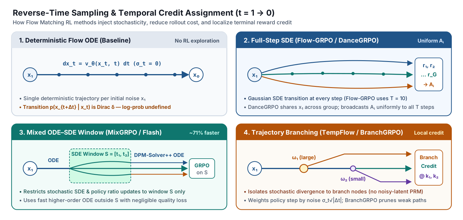
Why cannot we simply plug GRPO into a pre-trained Rectified Flow model out of the box? Because Flow Matching generates samples via the deterministic probability flow ODE $dx_t = v_\theta(x_t, t, c)\,dt$ ($t: 1 \to 0$), so a single initial noise $x_1$ produces one fixed trajectory and a degenerate Dirac-delta transition $p_\theta(x_{t+\Delta t} \mid x_t, c) = \delta(x_{t+\Delta t} - \Phi(x_t))$. That removes both prerequisites of policy-gradient RL at once:
- No stochastic exploration: a fixed seed produces zero rollout diversity to rank better vs. worse generations for the same prompt.
- Intractable transition density: the policy log-probability $\log \pi_\theta(a_t \mid s_t)$ is undefined.
Marginal-Preserving SDE Derivation
Flow-GRPO[12] resolves this cleanly by converting the deterministic ODE into a stochastic differential equation (SDE) whose marginal density $p_t(x)$ matches the original flow model at every time $t \in [0, 1]$[11].
Step 1: Forward Fokker–Planck equivalence. Under forward noising time ($t: 0 \to 1$), the flow ODE velocity $v_t$ preserves $p_t$ via the Continuity Equation $\partial_t p_t + \nabla\cdot(p_t v_t) = 0$. Now consider a forward Itô SDE $dx_t = f_t^{\text{fwd}}(x_t)\,dt + \sigma_t\,dw_t$, whose marginal density evolves according to the Fokker–Planck equation:
$$\frac{\partial p_t}{\partial t} + \nabla\cdot(p_t f_t^{\text{fwd}}) = \frac{1}{2}\sigma_t^2 \Delta p_t = \nabla\cdot\!\left(\frac{\sigma_t^2}{2}\nabla p_t\right) = \nabla\cdot\!\left(\frac{\sigma_t^2}{2}p_t\nabla\log p_t\right)$$Matching $\nabla\cdot(p_t v_t) = \nabla\cdot(p_t f_t^{\text{fwd}} - \frac{\sigma_t^2}{2}p_t\nabla\log p_t)$ gives the marginal-preserving forward drift $f_t^{\text{fwd}}(x_t) = v_t(x_t) + \frac{\sigma_t^2}{2}\nabla\log p_t(x_t)$.
Step 2: Anderson time-reversal ($t: 1 \to 0$). By Anderson's reverse-time SDE theorem, reversing a forward SDE with drift $f_t^{\text{fwd}}$ and diffusion $\sigma_t$ subtracts $\sigma_t^2\nabla\log p_t(x_t)$ from the drift:
$$dx_t = \Big(f_t^{\text{fwd}}(x_t) - \sigma_t^2 \nabla\log p_t(x_t)\Big)dt + \sigma_t\,d\bar w_t = \left[v_t(x_t) - \frac{\sigma_t^2}{2}\nabla\log p_t(x_t)\right]dt + \sigma_t\,d\bar w_t$$Intuitively, as time flows backward from noise ($t=1$) toward data ($t=0$), $dt \lt 0$, so $-\frac{\sigma_t^2}{2}\nabla\log p_t(x_t)\,dt$ pushes the trajectory upward along the log-density gradient to counteract the random diffusion $\sigma_t\,d\bar w_t$.
Step 3: Expressing the score via the flow velocity. For Rectified Flow linear interpolation $x_t = (1-t)x_0 + t x_1$ with $x_1 \sim \mathcal{N}(0, I)$, the conditional transition is Gaussian $p(x_t \mid x_0) = \mathcal{N}((1-t)x_0, t^2 I)$. Thus $\nabla_{x_t}\log p(x_t \mid x_0) = -\frac{x_t - (1-t)x_0}{t^2} = -\frac{x_1}{t}$, and taking conditional expectation via Tweedie's identity yields $\nabla\log p_t(x_t) = -\frac{\mathbb{E}[x_1 \mid x_t]}{t}$. Meanwhile, the optimal velocity satisfies $v_t(x_t) = \mathbb{E}[x_1 - x_0 \mid x_t]$ alongside $x_t = (1-t)\mathbb{E}[x_0 \mid x_t] + t\,\mathbb{E}[x_1 \mid x_t]$, which eliminates $\mathbb{E}[x_0 \mid x_t]$ to give $\mathbb{E}[x_1 \mid x_t] = x_t + (1-t)v_t(x_t)$. Substituting yields the exact score–velocity identity:
$$\nabla \log p_t(x_t) = -\frac{1}{t}\Big(x_t + (1-t)v_t(x_t)\Big)$$Step 4: Euler–Maruyama discretization and closed-form KL. Plugging the score identity into the reverse SDE and discretizing with negative step $\Delta t = t_{\text{prev}} - t \lt 0$ (moving from $t$ to $t+\Delta t$) gives the Gaussian policy transition $\pi_\theta(x_{t+\Delta t} \mid x_t, c) = \mathcal{N}(\mu_\theta(x_t, t),\, \sigma_t^2 |\Delta t|\,I)$:
$$x_{t+\Delta t} = \underbrace{x_t + \left[v_\theta(x_t, t) + \frac{\sigma_t^2}{2t}\big(x_t + (1-t)v_\theta(x_t, t)\big)\right]\Delta t}_{\mu_\theta(x_t, t)} + \sigma_t\sqrt{|\Delta t|}\,\epsilon, \qquad \epsilon \sim \mathcal{N}(0, I)$$Factoring $x_t$ and $v_\theta(x_t, t)$ inside $\mu_\theta$ gives the exact form implemented in Diffusers schedulers:
$$\mu_\theta(x_t, t) = x_t\left(1 + \frac{\sigma_t^2}{2t}\Delta t\right) + v_\theta(x_t, t)\left(1 + \frac{\sigma_t^2(1-t)}{2t}\right)\Delta t$$With noise schedule $\sigma_t = a\sqrt{\frac{t}{1-t}}$ (where $a$ is a scalar noise-level hyperparameter), both $\pi_\theta$ and $\pi_{\text{ref}}$ share identical isotropic variance $\sigma_t^2 |\Delta t| I$. Their step-wise KL divergence therefore reduces to a closed-form weighted $L_2$ distance between velocity predictions—no Monte Carlo estimation needed:
$$D_{\text{KL}}(\pi_\theta \,\|\, \pi_{\text{ref}}) = \frac{\|\mu_\theta - \mu_{\text{ref}}\|^2}{2\sigma_t^2 |\Delta t|} = \frac{|\Delta t|}{2}\left(\frac{1}{\sigma_t} + \frac{\sigma_t(1-t)}{2t}\right)^2 \|v_\theta(x_t, t) - v_{\text{ref}}(x_t, t)\|^2$$Implementing sde_step_with_logprob in PyTorch
In the official yifan123/flow_grpo codebase, a single patched scheduler function sde_step_with_logprob handles both trajectory sampling during rollout (when prev_sample=None) and exact log-probability re-evaluation during GRPO policy updates (when prev_sample is fed back from the replay buffer):
def sde_step_with_logprob(
    self,
    model_output: torch.FloatTensor,   # v_theta(x_t, t, c)
    timestep: Union[float, torch.Tensor],
    sample: torch.FloatTensor,         # current latent x_t
    noise_level: float = 0.7,
    prev_sample: Optional[torch.FloatTensor] = None,
    generator: Optional[torch.Generator] = None,
):
    model_output = model_output.float()
    sample = sample.float()
    if prev_sample is not None:
        prev_sample = prev_sample.float()

    # Map discrete scheduler timestep to continuous sigma schedule t in [0, 1]
    step_index = [self.index_for_timestep(t) for t in timestep]
    prev_step_index = [step + 1 for step in step_index]
    sigma = self.sigmas[step_index].view(-1, *([1] * (sample.ndim - 1)))
    sigma_prev = self.sigmas[prev_step_index].view(-1, *([1] * (sample.ndim - 1)))
    sigma_max = self.sigmas[1].item()  # guard 1 / (1 - sigma) singularity at sigma = 1

    dt = sigma_prev - sigma  # strictly negative during denoising (1 -> 0)
    std_dev_t = torch.sqrt(sigma / (1 - torch.where(sigma == 1, sigma_max, sigma))) * noise_level

    # Marginal-preserving SDE drift mean: mu_theta(x_t, t)
    prev_sample_mean = (
        sample * (1 + std_dev_t**2 / (2 * sigma) * dt)
        + model_output * (1 + std_dev_t**2 * (1 - sigma) / (2 * sigma)) * dt
    )

    # Mode 1 (Rollout): sample next latent x_{t+dt}; Mode 2 (Update): score stored transition
    if prev_sample is None:
        variance_noise = randn_tensor(
            model_output.shape, generator=generator, device=model_output.device, dtype=model_output.dtype
        )
        prev_sample = prev_sample_mean + std_dev_t * torch.sqrt(-1 * dt) * variance_noise

    # Isotropic Gaussian transition log-prob (averaged over latent dimensions for ratio stability)
    step_std = std_dev_t * torch.sqrt(-1 * dt)
    log_prob = (
        -((prev_sample.detach() - prev_sample_mean) ** 2) / (2 * (step_std**2))
        - torch.log(step_std)
        - torch.log(torch.sqrt(2 * torch.as_tensor(math.pi, device=sample.device)))
    )
    log_prob = log_prob.mean(dim=tuple(range(1, log_prob.ndim)))
    return prev_sample, log_prob, prev_sample_mean, std_dev_t
Four engineering subtleties in this snippet matter directly in practice:
- Sign of
dt: Becausesigma_prev < sigmaalong the reverse schedule,dtis negative; multiplying by-1 * dtinsidetorch.sqrtgives $|\Delta t|$, while the drift term uses signeddtso $x_t$ moves toward clean data. - Boundary singularity guard: At the very first step $t = \sigma = 1$, $\sqrt{\sigma/(1-\sigma)}$ divides by zero;
torch.where(sigma == 1, sigma_max, sigma)cleanly caps it at the second schedule grid point. - Detach on
prev_sample: During optimization, gradients flow exclusively throughprev_sample_mean(i.e., $v_\theta$), treating the realized latent transitionprev_sampleas a fixed action sample. - Per-dimension mean vs. raw sum: Averaging
log_probacross $(C, H, W)$ instead of summing tens of thousands of latent coordinates prevents $\exp(\log\pi_\theta - \log\pi_{\text{old}})$ from underflowing or exploding immediately to clipping bounds.
Reverse-Process Flow-GRPO Family
Once sde_step_with_logprob unlocks step-level policy gradients for continuous flows, an entire ecosystem of methods emerged to scale it across modalities, slash rollout cost, fix temporal credit assignment, and prevent reward hacking.
Flow-GRPO and DanceGRPO: Establishing the Online RL Baseline
Flow-GRPO[12] pairs the ODE-to-SDE conversion above with a simple but decisive systems optimization: Denoising Reduction. Running 40 SDE steps during every RL training iteration is prohibitively slow, yet Flow-GRPO shows that trajectories collected with a coarse $T=10$ SDE schedule still provide strong, informative reward rankings for policy updates—while test-time inference keeps the full $T=40$ deterministic ODE schedule to preserve high visual fidelity. Combined with closed-form KL regularization to curb reward hacking, Flow-GRPO delivered sharp gains on SD3.5 across compositional generation (GenEval), visual text rendering (OCR), and human preference benchmarks.
DanceGRPO[13] generalizes the same SDE-MDP formulation into a unified visual RL engine spanning both diffusion and rectified-flow backbones (SD1.4, FLUX, HunyuanVideo, SkyReels-I2V) across text-to-image, text-to-video, and image-to-video synthesis. Optimizing the clipped group-relative objective across $G$ trajectories and $T$ steps:
$$J_{\text{DanceGRPO}}(\theta) = \mathbb{E}_{\{o_i\}_{i=1}^G \sim \pi_{\theta_{\text{old}}}}\!\left[\frac{1}{G}\sum_{i=1}^G \frac{1}{T}\sum_{t=1}^T \min\!\Big(\rho_{i,t}(\theta)\widehat A_i,\, \operatorname{clip}(\rho_{i,t}(\theta), 1-\epsilon, 1+\epsilon)\widehat A_i\Big)\right]$$DanceGRPO isolates four practical engineering recipes that determine whether large-scale visual RL converges cleanly:
- Shared initialization noise: Unlike earlier diffusion RL work (e.g., DDPO) that sampled independent initial latents $x_1$ for every rollout, DanceGRPO initializes all $G$ samples in a prompt group from the same $x_1$—so variance comes purely from intermediate SDE exploration rather than lucky/unlucky starting noise, dramatically lowering variance.
- Timestep subsampling: Only a subset of denoising steps needs gradient updates per iteration, cutting backward-pass compute with minimal quality impact.
- Multi-reward ensembling: Optimizing a single preference score (such as HPS-v2.1 alone) causes over-saturated, "oily" textures; pairing aesthetic rewards with semantic alignment (e.g., CLIP / VLM judges) balances fidelity and visual naturalness.
- Omitting KL + Best-of-$N$ alignment: Under shared noise and multi-reward stabilization, DanceGRPO finds that dropping the explicit KL term does not destabilize training and lifts final alignment; pairing with Best-of-$N$ selection further accelerates high-reward convergence.
MixGRPO, TempFlow-GRPO, and BranchGRPO: Efficiency and Temporal Credit
Despite strong results, full-trajectory SDE RL suffers from two structural flaws:
- High rollout and re-evaluation cost: computing ratios across all $T$ steps requires running both $\pi_\theta$ and $\pi_{\text{old}}$ over the entire denoising chain.
- Temporal uniformity assumption: broadcasting a single sparse terminal reward $r(x_0, c)$ equally to every step ignores the physical reality that early high-noise steps govern global layout while late low-noise steps refine fine texture.
MixGRPO[14] attacks the cost bottleneck with a mixed ODE–SDE sliding window. Rather than injecting noise everywhere, it restricts stochastic SDE sampling—and thus MDP policy evaluation and GRPO updates—to a moving sub-interval $S = [t_1, t_2]$ that sweeps across the denoising horizon, while keeping deterministic ODE integration outside $S$:
$$dx_t = \begin{cases} \left[v_\theta(x_t, t) - \frac{\sigma_t^2}{2}\nabla\log p_t(x_t)\right]dt + \sigma_t\,d\bar w_t, & t \in S \\ v_\theta(x_t, t)\,dt, & t \notin S \end{cases}$$Because steps outside $S$ never require transition log-probabilities, MixGRPO-Flash swaps Euler ODE outside the window for higher-order solvers like DPM-Solver++, cutting training time by up to ~71% while preserving or improving HPS-v2.1, PickScore, ImageReward, and UnifiedReward metrics.
TempFlow-GRPO[15] directly tackles temporal uniformity through two complementary mechanisms:
- Trajectory Branching for Process Credit: Evaluating intermediate noisy latents $x_t$ with a learned Process Reward Model (PRM) is unreliable because partially denoised features lack clear semantics. Instead, TempFlow-GRPO runs deterministic ODE up to a chosen branch step $k$, injects a single stochastic SDE fork $x_{k+\Delta t} = \text{SDE}(x_k, \epsilon)$ to generate distinct branches, and completes every branch deterministically via ODE to clean images $x_0$. By Credit Localization, all variance in final terminal rewards across branches is strictly attributable to the policy's decision at step $k$—yielding exact process credit from standard terminal reward models alone.
- Noise-Aware Policy Weighting: Measuring reward standard deviation across timesteps confirms that exploration variance peaks early (high noise $\sigma_t$) and decays toward zero near $t \to 0$. TempFlow-GRPO scales each timestep's clipped objective by its normalized SDE noise magnitude $\operatorname{Norm}(\sigma_t\sqrt{|\Delta t|})$:
This gives early structural steps strong learning pressure for global layout exploration while letting low-noise refinement steps perform gentle, stable adjustments.
BranchGRPO[16] generalizes single-node branching into a structured prefix-sharing rollout tree: trajectories reuse shared deterministic prefixes, fork selectively across high-leverage depths, compute parent-relative advantages at tree edges, and prune unpromising branches early—trimming diffusion RL runtime by up to ~55% while tightening credit assignment.
Stabilizing Rewards and Ratios: Pref-GRPO, GRPO-Guard, and Flow-CPS
A parallel cluster of late-2025 refinements targets the statistical failure modes of group-normalized SDE RL:
- Pref-GRPO[17] notes that when a pointwise reward model assigns nearly indistinguishable scores to $G$ images in a group, dividing by $\operatorname{std}(\mathbf{R})$ blows up tiny scorer noise into huge gradients and triggers illusory reward hacking. Replacing pointwise scoring with a Pairwise Preference Reward Model (PPRM) and deriving advantages from within-group win rates stabilizes text-to-image RL substantially.
- GRPO-Guard[18] analyzes importance ratio distribution shifts across timesteps on FLUX.1-dev and SD3.5-M, discovering that uncalibrated clipping causes implicit over-optimization (generating degraded artifacts even as proxy reward climbs); introducing noise-condition-regulated clipping bounds prevents ratio drift.
- Flow-CPS[19] improves the discretization itself via Coefficients-Preserving Sampling, keeping exact marginal variance under coarse SDE step counts without brittle noise-level retuning.
Beyond Reverse-SDE: Forward-Process, Optimal Control, and Control Policies
Even with sliding windows and branching trees, reverse-SDE methods remain tethered to discretized Gaussian transition densities and backward step tracking. A major conceptual shift in late 2025 and 2026 asks: must RL happen inside the reverse SDE chain at all?
DiffusionNFT: Online RL Directly on the Forward Process
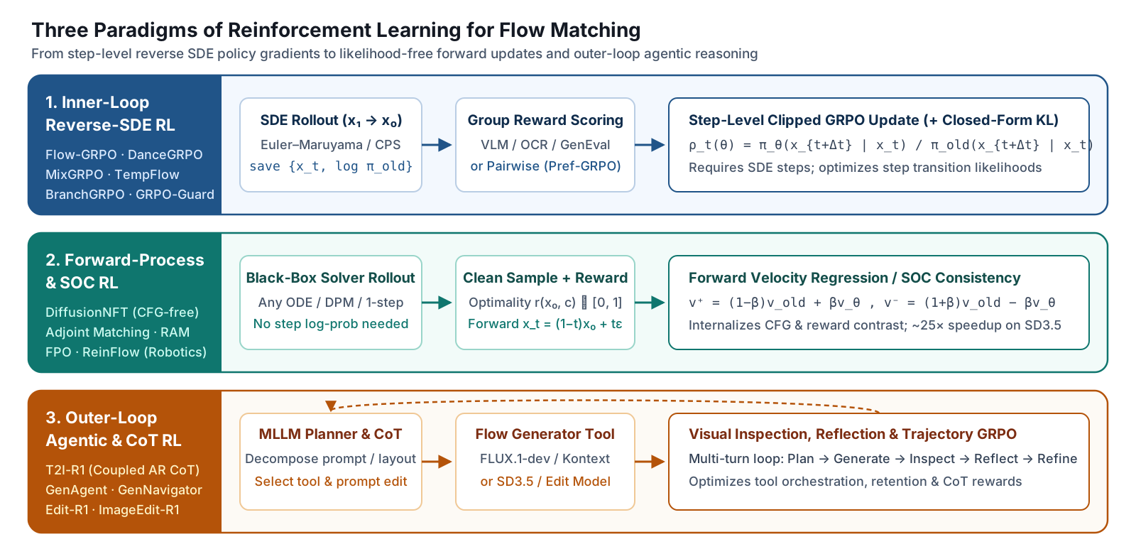
DiffusionNFT[20] breaks free from reverse-SDE restrictions entirely. Traditional rejection-sampling fine-tuning (RFT) discards half the rollouts—training only on high-reward images—which leaves the model blind to failure modes and prone to reward collapse. DiffusionNFT instead runs online rollouts using any black-box sampler (high-order ODE, few-step solver, or CFG-free inference), scores clean images with a normalized optimality reward $r(x_0, c) \in [0, 1]$, and optimizes the network directly on the forward flow-matching interpolation $x_t = (1-t)x_0 + t\epsilon$ with target velocity $\epsilon - x_0$.
Its central insight is an implicit parameterization around the old/reference policy $v^{\text{old}}$ with update strength $\beta \gt 0$:
$$v_\theta^+(x_t, t, c) = (1 - \beta)\,v^{\text{old}}(x_t, t, c) + \beta\,v_\theta(x_t, t, c), \qquad v_\theta^-(x_t, t, c) = (1 + \beta)\,v^{\text{old}}(x_t, t, c) - \beta\,v_\theta(x_t, t, c)$$Given clean rollout $(x_0, c)$ and optimality score $r(x_0, c) \in [0, 1]$, DiffusionNFT minimizes the negative-aware forward regression loss:
$$\mathcal{L}_{\text{NFT}}(\theta) = \mathbb{E}_{(x_0, c) \sim \pi_{\text{old}},\, t,\, \epsilon}\!\left[r(x_0, c)\,\big\|v_\theta^+(x_t, t, c) - (\epsilon - x_0)\big\|^2 + \big(1 - r(x_0, c)\big)\,\big\|v_\theta^-(x_t, t, c) - (\epsilon - x_0)\big\|^2\right]$$Look closely at the geometry: $v_\theta^+ - v_\theta^- = 2\beta(v_\theta - v^{\text{old}})$, which is mathematically isomorphic to Classifier-Free Guidance (CFG)—except instead of contrasting conditional vs. unconditional predictions at double inference cost, DiffusionNFT contrasts high-reward vs. low-reward trajectories during training and internalizes preference guidance directly into a single CFG-free velocity field!
Because forward regression needs no step log-probabilities and avoids forward–reverse discretization mismatch, DiffusionNFT achieves up to a $25\times$ efficiency speedup over Flow-GRPO, lifting SD3.5-Medium on GenEval from $0.24$ to $0.98$ within ~1k steps using a clean two-stage, five-reward curriculum:
- Stage 1 (Model-based preference): Jointly optimize PickScore, CLIPScore, and HPSv2.1 on Pick-a-Pic prompts to instill human aesthetics and prompt alignment.
- Stage 2 (Rule-based verifiers): Add verifiable GenEval and OCR rewards to sharpen spatial counting, attribute binding, and text rendering without losing visual quality.
Stochastic Optimal Control and Embodied Flow Policies
Two closely related lines—Stochastic Optimal Control (SOC) in generative modeling and continuous flow policies in robotics—converged independently on the exact same mathematical divide between noise injection and forward-loss surrogates:
- Adjoint Matching: formulates KL-regularized flow fine-tuning as a memoryless SOC problem via regression onto an adjoint ODE without differentiating through the full sampling chain[21], though originally requiring reward gradients $\nabla_{x_0} r(x_0)$.
- Reinforce Adjoint Matching (RAM): combines adjoint-matching optimality with a REINFORCE identity[22], yielding a pure consistency-regression loss that scales to non-differentiable rewards (VLM judges, OCR) on SD3.5 with neither backward adjoint sweeps nor step-wise importance ratios.
- ReinFlow (Embodied Flow RL): injects learnable noise networks into deterministic Rectified Flow and Shortcut action policies[23] to obtain discrete-time Markov chains with exact transition log-probs—mirroring Flow-GRPO for 1–4 step robotic control.
- FPO (Flow Policy Optimization): avoids exact likelihoods altogether by replacing the log-ratio in PPO-clip with an ELBO surrogate derived directly from the conditional flow matching (CFM) loss[24]—mirroring DiffusionNFT and RAM in continuous control.
From Single-Pass Denoising to Reasoning and Agentic RL
All methods in Sections 2 and 3 optimize the inner loop of a single forward generation pass. Yet complex compositional prompts ("three red cubes stacked left of a handwritten chalkboard sign") or multi-constraint image editing tasks often exceed what a single 28-step velocity pass can plan reliably without explicit decomposition, visual inspection, and iterative repair. This motivated a second frontier: bringing LLM-style Chain-of-Thought (CoT) and Agentic RL to visual synthesis.
Coupled Reasoning and Generation: T2I-R1 and Autoregressive CoT
T2I-R1[25] pioneered R1-style reasoning in unified multimodal models (built on Janus-Pro) via two coupled levels of CoT trained jointly with BiCoT-GRPO:
- Semantic-level CoT: Cold-started on GPT-4o reasoning traces, the language side plans object layout, visual attributes, and spatial relations in text before emitting any image tokens.
- Token-level CoT: The autoregressive visual head generates discrete image patches token-by-token conditioned on the semantic plan.
Both stages are reinforced jointly using an ensemble of four complementary rewards: (a) Human Preference Models (HPS, ImageReward) for aesthetics, (b) Object Detectors (GroundingDINO, YOLO-World) verifying presence and spatial position, (c) VQA Models (LLaVA) auditing attribute binding, and (d) a fine-tuned multimodal Output Reward Model (LLaVA-OneVision). Related autoregressive models such as ReasonGen-R1[26] and GoT-R1[27] adopt the same single-policy coupled SFT + GRPO recipe.
From an architectural standpoint, however, treating autoregressive image-patch emission as "token-level CoT" is something of a convenient abstraction: discrete AR generators still lag behind continuous Flow Matching Diffusion Transformers like FLUX.1-dev and SD3.5 in photorealism, typography, and local spatial precision. This raises a natural question: can we keep continuous Flow Matching models as the visual engine while still training an RL policy to reason, inspect, and iterate?
Agentic RL with Flow Matching Generators
Rather than forcing a single transformer to emit both reasoning text and discrete visual tokens, recent Agentic RL systems decouple cognition and rendering—treating continuous Flow Matching generators and editors as invokable tools inside a multi-turn closed-loop MDP:
- GenAgent (Multi-Turn Tool Use): frames text-to-image synthesis as an agentic Plan → Generate → Inspect → Reflect → Refine trajectory[28]: an MLLM core agent invokes FLUX.1-dev and local editing tools, inspects intermediate renders, diagnoses missing objects or broken bindings, and executes targeted refinements via cold-start SFT + Agentic RL.
- Generation Navigator (PRE-GRPO): models multi-turn generation as a state-conditioned MDP optimized with trajectory-level PRE-GRPO[29], balancing peak visual quality, cross-turn attribute retention, and iteration budget.
- UniWorld-V2 / Edit-R1 (CoT Reward Editing): addresses missed local edits and background drift under scalar scorers[30] by pairing a Chain-of-Thought Reasoning Reward Model (verifying decomposed edit checks) with DiffusionNFT updates on flow editors.
- ImageEdit-R1 (Multi-Agent Planner): trains a GRPO-optimized multi-agent orchestrator[31] that decomposes compound editing requests into ordered atomic calls executed by flow models.
- Reflect-DiT (In-Context Reflection): bridges inner and outer loops by feeding previous candidate images and textual VLM critiques directly as in-context conditioning to Diffusion Transformers[32], outperforming blind Best-of-$N$ search.
Taken together, inner-loop RL (Flow-GRPO, DiffusionNFT, RAM) and outer-loop Agentic RL (GenAgent, ImageEdit-R1) are complementary layers rather than competitors: inner-loop RL raises the single-shot ceiling of the continuous velocity field, while outer-loop Agentic RL supplies deliberate planning, tool orchestration, and error recovery over multi-step visual tasks.
Landscape Comparison and Practical Takeaways
The table below contrasts the representative methods across sampling assumptions, credit granularity, regularization, and ideal deployment regimes:
| Method | Paradigm | Solver Freedom | Credit Granularity | KL / CFG Handling | Best Fit |
|---|---|---|---|---|---|
Flow-GRPO |
Reverse-SDE GRPO | Euler SDE ($T=10$ train) | Uniform across all $T$ steps | Closed-form velocity KL | General T2I alignment baseline on SD3.5 |
DanceGRPO |
Unified SDE GRPO | Euler SDE + shared $x_1$ | Subsampled steps, uniform $A_i$ | KL omitted; multi-reward | Large-scale T2I / T2V / I2V (FLUX, HunyuanVideo) |
MixGRPO / Flash |
Mixed ODE–SDE window | SDE in $S$, DPM++ outside | Localized to sliding window $S$ | Clipped GRPO on $S$ | Cutting reverse-SDE wall-clock cost (~71%) |
TempFlow-GRPO |
Branching + noise weight | ODE + SDE branch forks | Exact node + $\sigma_t\sqrt{|\Delta t|}$ weight | Noise-aware clipped GRPO | Fine-grained layout vs. detail credit |
BranchGRPO |
Prefix-tree branching | Shared-prefix tree SDE | Parent-relative tree edges | Path pruning + GRPO | High-throughput trajectory exploration (~55% faster) |
Pref-GRPO / Guard |
Stabilized SDE GRPO | Reverse SDE | Pairwise win-rate / regulated | Regulated ratio clipping | Preventing reward hacking & ratio drift on FLUX |
DiffusionNFT |
Forward-process contrast | Any black-box solver | Direct forward FM regression | CFG-free ($v^+, v^-$) | Fastest single-pass alignment (~25× vs Flow-GRPO) |
RAM |
SOC consistency | Arbitrary sampler | Adjoint-REINFORCE loss | Built-in KL target | Non-differentiable rewards without SDE ratios |
T2I-R1 |
Coupled AR CoT GRPO | Autoregressive tokens | Semantic + token BiCoT | Multi-expert reward ensemble | Unified discrete MLLMs needing prompt CoT |
GenAgent / Edit-R1 |
Outer-loop Agentic RL | Wraps FLUX / Flow DiT | Multi-turn trajectory + CoT RRM | Trajectory RL / tool verify | Complex spatial layouts & multi-step editing |
In practice, choosing a Flow Matching RL stack comes down to four concrete rules of thumb:
- Prioritize forward-process or hybrid windows for compute efficiency: If you only need single-pass preference or verifier alignment and want fast turnaround without reverse-SDE plumbing, start with DiffusionNFT (bonus: CFG-free inference) or MixGRPO-Flash.
- Separate structural exploration from texture refinement: When full-trajectory SDE updates distort fine textures or converge slowly, adopt TempFlow-GRPO's noise-aware weighting or BranchGRPO's prefix-sharing tree so high-noise early steps do the heavy exploration.
- Guard against silent reward hacking early: Always share initial noise $x_1$ across prompt groups (DanceGRPO), combine aesthetic models with semantic/rule verifiers (OCR, GenEval), and replace noisy scalar differences with Pref-GRPO pairwise rankings or GRPO-Guard clipping whenever proxy scores outrun human visual quality.
- Add an outer Agentic RL loop when single-pass prompts hit a ceiling: When failure modes stem from spatial planning, multi-object counting, or iterative editing rather than per-step denoising fidelity, wrap your aligned Flow Matching model inside an MLLM planning-and-inspection agent (GenAgent, Generation Navigator, or ImageEdit-R1) instead of overloading the velocity field alone.
Citation
If you reference these notes or diagrams, please cite:
Chaoran Feng (2026). "Reinforcement Learning in Flow Matching Models". Chaoran Feng's Blog. https://www.falcary.com/blogs/flow-matching-rl/
@article{feng2026flowrl,
  title   = {Reinforcement Learning in Flow Matching Models},
  author  = {Feng, Chaoran},
  year    = {2026},
  month   = {September},
  url     = {https://www.falcary.com/blogs/flow-matching-rl/}
}
References
- Training Diffusion Models with Reinforcement Learning. Black, Janner, Du, Kostrikov, Levine, ICLR 2024 (arXiv:2305.13301).
- Proximal Policy Optimization Algorithms. Schulman, Wolski, Dhariwal, Radford, Klimov, 2017 (arXiv:1707.06347).
- Direct Preference Optimization: Your Language Model is Secretly a Reward Model. Rafailov, Sharma, Mitchell, Ermon, Manning, Finn, NeurIPS 2023 (arXiv:2305.18290).
- Diffusion Model Alignment Using Direct Preference Optimization. Wallace, Dang, Rafailov, Zhou, Lou, Purushwalkam, Ermon, Xiong, Joty, Naik, CVPR 2024 (arXiv:2311.12908).
- DeepSeekMath: Pushing the Limits of Mathematical Reasoning in Open Language Models. Shao, Wang, Zhu, Xu, Song, Bi, Zhang, Zhang, Li, Wu, Guo, 2024 (arXiv:2402.03300).
- Kimi k1.5: Scaling Reinforcement Learning with LLMs. Kimi Team, 2025 (arXiv:2501.12599).
- DAPO: An Open-Source LLM Reinforcement Learning System at Scale. Yu, Zhang, Zhu, Yuan, Zuo, Yue, et al., 2025 (arXiv:2503.14476).
- VAPO: Efficient and Reliable Reinforcement Learning for Advanced Reasoning Tasks. Yue, Yuan, Yu, Zuo, Zhu, Xu, et al., 2025 (arXiv:2504.05118).
- Group Sequence Policy Optimization. Zheng, Liu, Li, Chen, Yu, Gao, et al. (Qwen Team), 2025 (arXiv:2507.18071).
- On-Policy Distillation of Language Models: Learning from Self-Generated Mistakes. Agarwal, Vieillard, Stańczyk, Ramos, Geist, Bachem, ICLR 2024 (arXiv:2306.13649).
- Score-Based Generative Modeling through Stochastic Differential Equations. Song, Sohl-Dickstein, Kingma, Kumar, Ermon, Poole, ICLR 2021 (arXiv:2011.13456).
- Flow-GRPO: Training Flow Matching Models via Online RL. Liu, Liu, Liang, Li, Liu, Wang, Wan, Zhang, Ouyang, NeurIPS 2025 (arXiv:2505.05470).
- DanceGRPO: Unleashing GRPO on Visual Generation. Xue, Wu, Gao, Kong, Zhu, Chen, Liu, Liu, Guo, Huang, Luo, 2025 (arXiv:2505.07818).
- MixGRPO: Unlocking Flow-based GRPO Efficiency with Mixed ODE-SDE. Li, Cui, Huang, Ma, Fan, Yang, Zhong, ECCV 2026 (arXiv:2507.21802).
- TempFlow-GRPO: When Timing Matters for GRPO in Flow Models. He, Fu, Zhao, Li, Yang, Yin, Rao, Zhang, 2025 (arXiv:2508.04324).
- BranchGRPO: Stable and Efficient GRPO with Structured Branching in Diffusion Models. Li, Wang, Zhu, Zhao, Lu, She, Zhang, ICLR 2026 (arXiv:2509.06040).
- Pref-GRPO: Pairwise Preference Reward-based GRPO for Stable Text-to-Image Reinforcement Learning. Wang, Li, Zang, Zhou, Bu, Wang, Lu, Jin, Wang, 2025 (arXiv:2508.20751).
- GRPO-Guard: Mitigating Implicit Over-Optimization in Flow Matching via Regulated Clipping. Wang, Liang, Liu, Liu, Liu, Zheng, Pang, Ma, Xie, Wang, Wang, Wan, Liang, 2025 (arXiv:2510.22319).
- Coefficients-Preserving Sampling for Reinforcement Learning with Flow Matching. Wang, Yu, 2025 (arXiv:2509.05952).
- DiffusionNFT: Online Diffusion Reinforcement with Forward Process. Zheng, Chen, Ye, Wang, Zhang, Jiang, Su, Ermon, Zhu, Liu, ICLR 2026 Oral (arXiv:2509.16117).
- Adjoint Matching: Fine-tuning Flow and Diffusion Generative Models with Memoryless Stochastic Optimal Control. Domingo-Enrich, Drozdzal, Karrer, Chen, ICLR 2025 (arXiv:2409.08861).
- Reinforce Adjoint Matching: Scaling RL Post-Training of Diffusion and Flow-Matching Models. Bergmeister, Jegelka, Nüsken, Domingo-Enrich, Pidstrigach, 2026 (arXiv:2605.10759).
- ReinFlow: Fine-tuning Flow Matching Policy with Online Reinforcement Learning. Zhang, Yu, Su, Wang, NeurIPS 2025 (arXiv:2505.22094).
- Flow Matching Policy Gradients. McAllister, Ge, Yi, Kim, Weber, Choi, Feng, Kanazawa, 2025 (arXiv:2507.21053).
- T2I-R1: Reinforcing Image Generation with Collaborative Semantic-level and Token-level CoT. Jiang, Guo, Zhang, Zong, Li, Zhuo, Yan, Heng, Li, 2025 (arXiv:2505.00703).
- ReasonGen-R1: CoT for Autoregressive Image Generation Models through SFT and RL. Zhang, Li, Yang, Wang, Yang, Qi, Bao, Chen, Luo, Qiu, 2025 (arXiv:2505.24875).
- GoT-R1: Unleashing Reasoning Capability of Autoregressive Visual Generation with Reinforcement Learning. Duan, Fang, Wang, Wang, Huang, Zeng, Li, Liu, 2025 (arXiv:2505.17022).
- GenAgent: Scaling Text-to-Image Generation via Agentic Multimodal Reasoning. Jiang, Wang, Zhou, Li, Liu, Xie, Chen, Zheng, Zhang, ECCV 2026 (arXiv:2601.18543).
- Generation Navigator: A State-Aware Agentic Framework for Image Generation. Liu, Feng, Wang, Zeng, Jin, 2026 (arXiv:2605.17969).
- UniWorld-V2: Reinforce Image Editing with Diffusion Negative-aware Finetuning and MLLM Implicit Feedback. Li, Liu, Zhang, Lin, Wu, Yuan, Yan, Ye, Yu, Niu, Wang, Cheng, Yuan, 2025 (arXiv:2510.16888).
- ImageEdit-R1: Boosting Multi-Agent Image Editing via Reinforcement Learning. Zhao, Ye, Liu, Shieh, Bui, 2026 (arXiv:2603.08059).
- Reflect-DiT: Inference-Time Scaling for Text-to-Image Diffusion Transformers via In-Context Reflection. Li, Kallidromitis, Gokul, Koneru, Kato, Kozuka, Grover, 2025 (arXiv:2503.12271).